Model
Optimizing enzyme ratios in the tagatose synthesis pathway
Introduction
According to the design, we introduced a reaction pathway into the peroxisome of the Yarrowia lipolytica to produce borneol. It is a multi-step reaction from acetyl coenzyme A to GPP, the precursor of borneol. The relative amount of enzymes, i.e., enzyme ratio, plays a critical role in driving the overall reaction. In order to maximize the yield of borneol to provide adequate raw material for the drug, here we build a kinetic model combining five reactions from acetyl coenzyme A to mevalonate diphosphate to predict the optimal enzyme ratio for the reactions.
Description
Let's start with the reaction pathway, cf. Fig. 1. In the peroxisome:
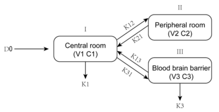
The Yarrowia lipolytica produces acetyl coenzyme A through the β-oxidation of fatty acids in the peroxisome. Acetyl coenzyme A is then used to produce the precursor of borneol in an eight-step reaction that we have introduced. It is known that there are not above reactions and corresponding side reactions in the peroxisome before engineering. Theoretically, increasing the yield of mevalonate diphosphate would facilitate the production of GPP. The yield of mevalonate diphosphate is strongly linked to the enzyme ratio in the upstream reactions. So, we will explore the optimal enzyme ratio for the production of mevalonate diphosphate in the following section.
First of all, we use Michaelis-menten equation to describe the kinetics of an enzymatic reaction:
The following symbols are used in our models:
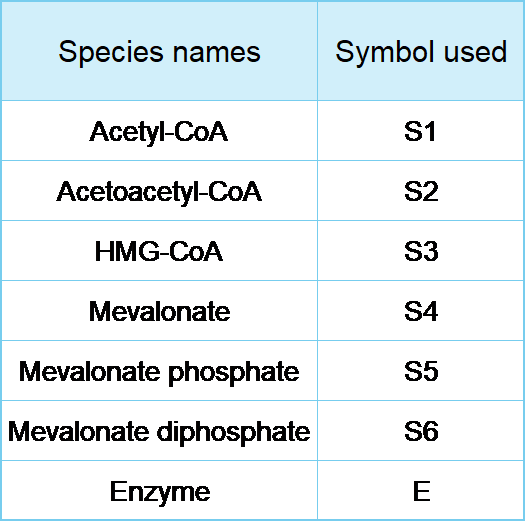
Reaction of the synthesis of S6 and its upstream reactions:
Reaction1:(E1)2S1 ⟺ S2+ CoA
forward reaction:

reverse reaction:

Reaction2:(E2)S2 + CoA ⟹ S3

Reaction3:(E3)S3 + 2NADPH + 2H+ ⟹ S4 + 2NADP+ + CoA

Reaction4:(E4) S4 + ATP ⟹ S5 + ADP

Reaction5:(E5) S5 + ATP ⟹ S6 + ADP

Reaction of S6 consumption:
Reaction6:(E6)S6+ ATP ⟹ S7 + Pi + CO2 + ADP

The above parameters can be found in subsection Parameters.
We ignore the reverse reactions of reactions 2 to 6 because their rate constants (k) are much smaller than forward reactions’. Using these rate equations, we can establish the relationship between the concentration of acetyl coenzyme A and the concentration of mevalonate diphosphate at certain enzyme ratio.
If we want to explore the optimal enzyme ratio for reactions, we need to assume a constant value for the sum of enzymes and then change the enzyme ratio to compare the yield of GPP at different ratios. Based on the Genetic Algorithm, we search for the optimal resolution by simulating the natural evolutionary process.
First, we set each enzyme to an initial value of 20 and fix the total number of enzymes to 120. We consider the relative content of the six enzymes as six genes and then code these genes into yeast ‘s “chromosome”. Each individual represents a solution for given problem.
Second, we assume that a yeast produces one yeast as a generation and that Simple Mutation occurs in every generation, which means that a variation operation is performed on the values of two randomly specified motifs in the coding string, i.e. the values of two enzymes are randomly changed while the total number of enzymes remains unchanged.
Third, for each offspring, we compare fitness with the previous generation and select. We decode the individual coding strings to obtain the phenotype, i.e. the enzyme ratio, and then we can calculate the corresponding S6 yield and compare the fitness of this generation with that of the previous generation. If it is higher than the fitness of the previous generation, we eliminate the previous generation and produce offspring based on this generation, otherwise we eliminate this generation and continue to produce offspring based on the previous generation.
Thus each successive generation is more suited for their environment, which means that the optimal enzyme ratio can be calculated eventually.
However, during the process, we found that if we used S6 yield directly as a function of fitness to compare yeast fitness, the reaction time steps would have to be within 1*10^ (-4) s in order to accurately obtain the concentration of the substrate in each reaction. Within a finite number of cycles, the program could only obtain S6 yield in a very short time, which couldn’t meet the yeast fermentation time designed.
So, we made some improvements and used mathematical proofs to convert the problem of comparing S6 concentrations at equilibrium into a problem of comparing the slope of the S6 concentration as a function of time, so that the program could predict the S6 concentration at equilibrium in a shorter time.
The following is the process of our proof.

S6 concentration derivative with respect to time:


When the concentration of S6 → +∞:

Since the S6 concentration actually cannot tend to infinity, so:

Solving the differential equation gives:

When t → +∞, the reaction reaches equilibrium and the concentration of S6 tends to a constant value, from which we can deduce the concentration of S6 at equilibrium:

Next, we prove that the greater the slope of the function of S6 concentration as a function of time, the greater the S6 equilibrium concentration.
Clearly, the S6 equilibrium concentration is monotonically increasing with respect to C1.
We consider S6 ,i.e. the slope at a concentration of S6 equal to half of the equilibrium concentration, when the slope has stabilised.


Derivation with respect to C1 gives:

Since the magnitude of C2 is around 10^(-6), we get:


So, the slope of the function of S6 concentration as a function of time is monotonically increasing with respect to C1.
Finally, we can conclude that the greater the slope of the function of S6 concentration as a function of time, the greater the equilibrium concentration of S6.
Based on this, our program can predict and compare the magnitude of the S6 equilibrium concentration by the change in S6 concentration over a shorter period of time, and thus get the optimum enzyme ratio more efficiently.
Results
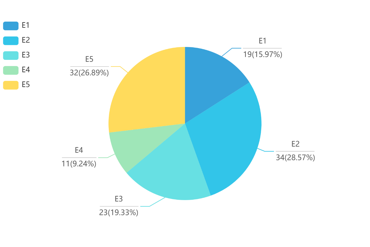
Parameters:
Here we are going to introduce our choice of parameters.
The following are the parameters that will be used in the rate equations.

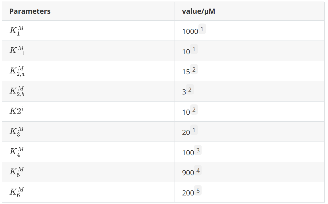
Considering that the carbon source of lipolytic yeast in the design is fatty acids and that the yeast peroxisome uses fatty acids for β-oxidation to produce relatively high concentration of acetyl coenzyme A, we considered the concentration of acetyl coenzyme A in the peroxisome as a constant value. The peroxisome is a relatively closed system and the major intermediates, end products and enzymes of our introduced reaction pathway were not present before the modification, so the initial S2 to S6 concentrations were 0. The enzyme concentrations for each reaction were on the order of μM.
Optimizing enzyme ratios in the tagatose synthesis pathway
enzyme ratio optimization

Fig.1.
Vmax=8.87mmol/s
Km = 0.51 mM
What follows are the constants for the Michaelis-Menten equation.
Vmax=225±13(nkat*mg-1)
Km = 25 ±4(mM)
So, if the estimate v=Vmax valid, the concentration of galactose is required to be over 100 Km(2.5mol·L-1) when v=0.99Vmax.
However, it is a concentration impossible to reach in vivo.
However, we did not find constants for RIGDH measured in an environment similar to the in vivo one, which is explained by the instability of NADH in lower pH.
And the Km is 8.8 mM, Kcat is 13.5 U under pH 9.0 and 37℃
According to the figure "Effect of pH on the activity of RIGDH", the activity of RIGDH is reduced to about 20%, consequently, we estimate Kcat to be 13.5 * 20% U under pH 6.5-7.0.
We employed an optimization algorithm that contains initiation, target function calculation, iteration with mutation, and result evaluation.
For initiation, we chose random distribution to initial the ratio of the enzymes. This initiation is done 50 or more times to create a group of particles, each representing a certain ratio. With this group of particles, we could achieve the effect of Particle Swam Optimization.
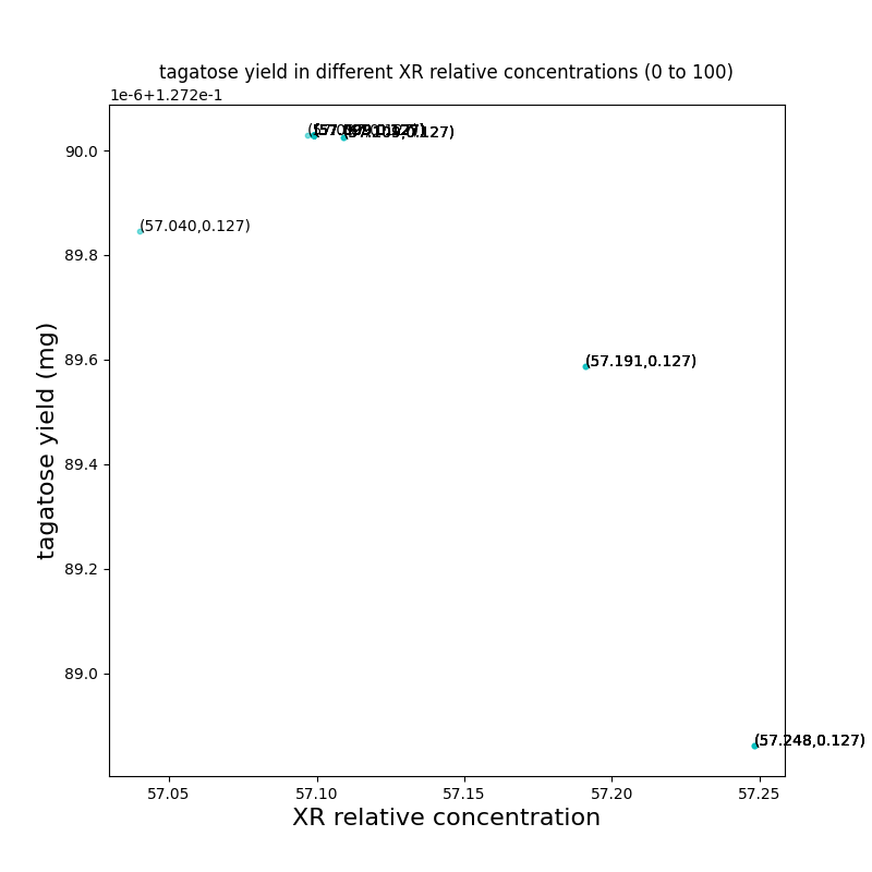
Then we consider the concentration of tagatose in a pre-determined time as the target value.
We iterate the ratio of enzymes in two ways. First, in a certain possibility, we made all of the particles move toward the best ratio in a recent situation. Otherwise, a random search is made to avoid being stuck to a local optimization.
We iterate about 50 times and plot the ratio of every particle as a result. A single particle's ratio change and corresponding target value were also plotted for observation.
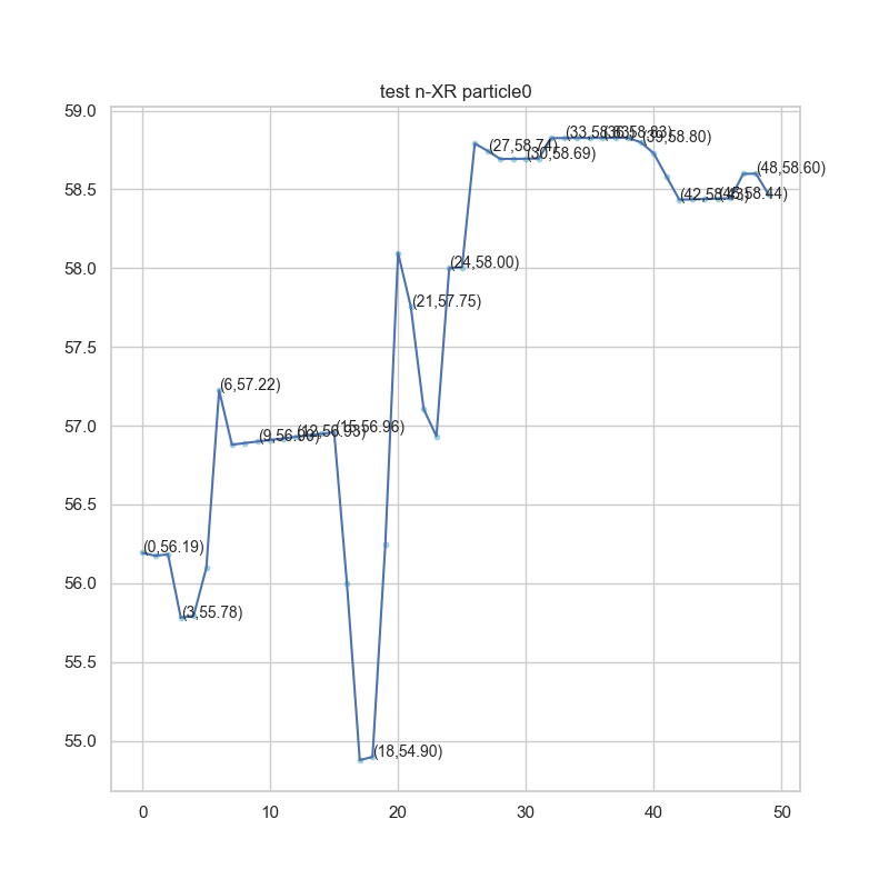
Fig.2.
