Why CAHS?
The cytosolic-abundant heat soluble protein (CAHS) from the tardigrade P. richtersi is another intrinsically disordered protein that prevents protein aggregation and retains protein functions under desiccation or freeze-thaw conditions. However, instead of employing the entropic bristle mechanism, the CAHS has a core region (residues 121-183) that associates with client proteins to block client proteins from aggregating with each other. Within the core region, motif 1 (residues 124-142) is the most critical for preventing client protein aggregation (Kang et al., 2024). Hence, the CAHS core region was selected as a solubilising protein (instead of a tag covalently linked to a client protein) for directed evolution, with an emphasis on motif 1, to further enhance its performance in preventing protein aggregation.
How we built the CAHS Library
Amino acid mutagenesis and filtering
For intrinsically disordered CAHS Core, it was documented that it prevents client protein-protein aggregation by adopting an amphiphilic α-helical conformation in motif 1 to protect aggregation-prone client protein such as lactate dehydrogenase(LDH) (Kang et al., 2024). Within the CAHS Core region, motif 1 (residues 124-142) has been identified as the most critical for this purpose. We therefore restricted mutagenesis to motif 1 and kept the remainder of the core region constant. The mechanisms by which the other regions contribute to the overall function are not well understood, so rational or randomised mutation there would be difficult to come up with and would risk disrupting activity without a clear basis for doing so. In doing so, this also concentrated the library’s diversity on the region most likely to influence performance.
CAHS1 Core (121--183): TEA[YRKQQEVEADKIRKELEKQ]HLRDVEFRKDIVEMAIENQKKMIDVESRYAKKDMDRERVKV

Motif 1 (124-142): YRKQQEVEADKIRKELEKQ
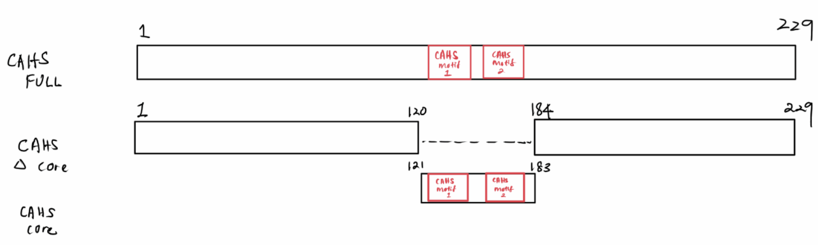
Figure 1. Schematic representation of where the residues are located, adapted from Kang et al., 2024.
Therefore, Pace & Scholtz sum was chosen as a lower sum indicates a better overall ability of forming such a helical conformation. Similarly, Pace & Scholtz mean was chosen to measure the same ability on a per residue basis (Pace & Scholtz, 1998). Pace and Scholtz values are a helix propensity scale that measures how easily each amino acid forms an alpha helix. Additionally, the number of proline residues in each mutant was counted, as more proline residues disrupts the helical conformation more due to its restriction in the Φ angle.
Moreover, the hydrophobic moment was chosen as a higher moment can potentially improve the ability of CAHS Core to use its hydrophobic side to associate with aggregation-prone patches of hydrophobic residues on surface of client proteins and to use its hydrophilic side to enhance solubility in aqueous cytosol. However, a very high hydrophobic moment may introduce antimicrobial properties into IDP as it causes bacterial membrane disruption (Zhang et al., 2025), and was therefore avoided. Similarly, the fraction of actual hydrophobic residues on the hydrophobic face of the CAHS helix (face occupancy) was chosen as a higher face occupancy may indicate more CAHS-client protein association that prevents aggregation.
Hence, each CAHS Core mutant was characterised with these chosen parameters. Then, the mutants were compared against the parameter values from the original CAHS Core sequence. Mutants that don’t meet the criteria listed below were discarded. Table 1 lists out the exact in-silico mutant selection criteria for each parameter.
Table 1: In silico selection criteria of CAHS mutants.
| Parameter | CAHS Criteria |
|---|---|
| Pace & Scholtz sum | ≤6.68 |
| Pace & Scholtz mean | ≤0.352 |
| Hydrophobic moment | ≥0.263, ≤0.526 |
| Face occupancy | ≥0.6 |
| Number of proline | ≤0 |
Overall, 11000 CAHS mutant sequences in the library were narrowed to 458 sequences after in-silico selection.
Encoding the library in degenerate DNA
Due to limitations on DNA sequence synthesis, we cannot synthesise the exact sequence for each of the selected sequences and mix them into a library. Instead, for each IDP, we compress its selected sequences into a representative DNA sequence with degenerate nucleotides to be synthesised. The degenerate sequence was generated using a customised program and can be accessed in https://github.com/TKA0329/iDEC_Cambridge_2026 .
The filtered CAHS Core sequences were deduplicated and aligned. Mutation hotspots were identified relative to the parental CAHS Core. Degenerate codons were chosen to cover the desired hotspot residues while penalising off-target residues and excluding stop-encoding codons.
The resulting 57-bp library sequence for motif 1, including the constant regions and excluding homology arms, was:
ACAGAAGCAAKRMKGARAMRAATGRVAARAGMAADGRRSARARTAAGAAAASAAWTGRMAAAAATGCACCTAAGAGACGTAGAATTCAGAAAAGACATAGTAGAAATGGCAATAGAAAACCAAAAAAAAATGATAGACGTAGAAAGCAGATACGCAAAAAAAGACATGGACAGAGAAAGAGTAAAAGTA
Its reported theoretical encoding space was 1741824 sequences. An estimated 47%, approximately 819319 sequences, met the computational criteria. These figures describe the designed encoding space, rather than the number successfully assembled, transformed or sequenced. Degenerate encoding also recombines allowed residues into sequences not present in the original filtered catalogue.
Expression and freeze-thaw cycles
We decided to express the variants as individual proteins instead of fused tags and subject the expressing E coli to repeated freeze-thaw cycles. Kang et al. (2024) reported that repeated freeze-thaw cycles lead to more aggregation of proteins, such as lactate dehydrogenase. Therefore, we reasoned that CAHS Core expressed in E coli can non-specifically protect various cytoplasmic proteins that are both aggregation-prone during repeated freeze-thaw and critical for E coli survival. This selection method is also high-throughput as it links the solubility-enhancing performance of CAHS Core mutants to the survival of E coli, and no individual measurement of solubility for each CAHS Core mutant is needed.
The degenerate CAHS Core IDP was split into two DNA fragments for synthesis: fragment 1 containing the motif 1 with degenerate nucleotides and fragment 2 containing only constant nucleotides. Fragment 1 was converted from single-stranded to double-stranded DNA using the protocol described in Tables 2 and 3 before assembly.
Table 2. Composition of reaction mixture for converting ssDNA degenerate IDP sequences to dsDNA.
| Component | Final concentration |
|---|---|
| Forward primer (IDP F, same as epPCR) | 0.5 μmol/L |
| Reverse primer (IDP R, same as epPCR) | 0.5 μmol/L |
| ssDNA degenerate IDP template | 0.1 mg/L |
| Q5®-XT Hot Start High-Fidelity 2X Master Mix (M2499S) | 1X (as defined by NEB M2499S) |
Table 3. Thermocycler program for 50 μL ssDNA to dsDNA conversion reaction mixture.
| Name | Temperature/℃ | Duration/sec | Repeat |
|---|---|---|---|
| Initial denaturation | 98 | 30 | 1 |
| Denaturation | 98 | 30 | 30 |
| Annealing | 61.7 | 20 | — |
| Extension | 72 | 7 | — |
| Preservation | 4 | — | 1 |
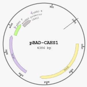
The molar ratio of the 3 components was 1:5:5. Linear-pBAD-no-sfGFP and fragment 2 were first incubated together for 30 minutes at 50 ℃, then fragment 1 was added and incubated further for 30 minutes. The product plasmid is the same as Figure 2, where CAHS1 becomes the degenerate CAHS IDP.
An alternative method of Gibson assembly was later developed using NEBuilder® HiFi DNA Assembly Master Mix (E2621S), where dsDNA linear-pBAD-no-sfGFP, ssDNA fragment motif 1 and dsDNA fragment 2 were added together in molar ratio 1:200:5 and incubated for 60 minutes at 50 ℃. The product plasmid was still the same as in Figure 2.
Figure 2. Map of annotated plasmid transformed into E coli for selection on CAHS Core IDP.
pBAD-CAHS1 libraries were then transformed into competent DH10β E. coli cells. For each library, 50ul frozen glycerol stocks of competent DH10β E. coli cells were thawed on ice, and 2μl of pBAD-IDP Gibson assembly products were added. The cells were rested on ice for 30 minutes, then subjected to heat shock at 42॰C for 30 seconds. The cells underwent recovery in SOC media for 1 hour before being incubated overnight in LB media culture. The expression of the CAHS Core variants was induced with 1% L-arabinose.
Repeated freeze-thaw selection
Flash freeze selection workflow
Induced cell culture suspensions containing the empty pBAD vector, CAHS Core derived library sequences and the wild type CAHS Core sequence were divided into 1.0 mL aliquots and subjected to 6 consecutive rounds of flash freeze selection, along with tubes that were not subjected to freeze-thaw selection (T0). For each cycle, each cell culture suspension was immersed in isopropanol/dry ice bath for 15 minutes to ensure complete freezing before being thawed at room temperature for 25 minutes. Cell culture suspensions were inspected visually between cycles to ensure complete thawing before the next stage of freezing and plated immediately after serial dilutions.
Deep freeze selection workflow
An additional freeze-thaw assay was performed, with cells frozen in a -70 °C freezer rather than the dry-ice/isopropanol cryogenic bath used in the flash-freeze assay.
Induced cell culture suspensions containing the empty pBAD vector, CAHS Core library sequences and the wild type CAHS Core sequences were divided into 0.5mL aliquots and subjected to deep freeze at –70 °C. Samples were frozen overnight with no strict timing due to no expected difference in mortality based on cumulative time spent frozen. (Sleight, Wigginton and Lenski, 2006) The cells were thawed for 45 minutes, serially diluted then plated. Colony count was used as a proxy for cell survival after selection.
Side note: Troubleshooting experiment for Desiccation
Originally, desiccation was our primary stress condition to test the effect of CAHS Core on E.coli’s survival in a desiccated state. The protocol for the dry run was as follows:
-
Sterile Whatman No.1 discs that were 6.5 mm in diameter were prepared with a hole puncher. 1.5 µL of the normalised cell suspension in saline was then pipetted onto each disc. The discs were then placed in a desiccator that contains desiccant.
-
After 30 minutes, the discs were then submerged in 5 ml LB Broth in a falcon tube. The tube was vortexed for 30 seconds to elute the cells off the filter. This was then plated. The experiment was repeated 3 times. Nevertheless, no colonies were observed the next day.
We hypothesised that it is because the bacteria were embedded in the filter paper and vigorous vortexing is unable to elute the cells off the paper. Filter papers in general have a pore size of approximately 11 µm, which is big compared to the size of a bacterial cell. When the suspension is applied and dried, the cells can migrate deep into the inner fibrous depths of the cellulose network and interact with the cellulose via a series of intermolecular interactions. Vortexing might not be able to flush the fluid completely out from the deep internal capillary pores. This hypothesis is untested. We then decided to explore other alternatives, like using a lyophilizer or other viable instruments, but these equipment is not readily accessible within the lab.
Excluding contaminating pBAD colonies
To distinguish putative library-containing colonies from an empty-vector background, cell suspensions were plated on agar supplemented with tetracycline and L-arabinose. The empty pBAD vector retained an arabinose-inducible sfGFP reporter, enabling colonies carrying this vector to be identified by fluorescence under UV illumination. Fluorescent colonies were excluded from colony counts used to assess the survival of the CAHS library. Non-fluorescent colonies were counted as putative insert-containing colonies; insert identity was not confirmed by colony PCR.
CALVADOS
To check that the selected variants had not gained a tendency to self-associate, we ran a coarse-grained CALVADOS simulation modelled loosely on the aggregation experiments of Kang et al., which measured the turbidity of CAHS Full, ΔCore and Core under varying protein concentrations and found that Full and ΔCore aggregated while Core did not. We simulated the same three constructs alongside a negative control (randomly reshuffled CAHS Core), our winner variant and worst performing variant in similar conditions (outlined below). Kang et al.’s result served as a positive-control benchmark: if the simulations reproduced the Full > ΔCore > Core ordering in terms of their aggregation-prone nature, with Full being the most aggregation-prone and Core being the least, they could be trusted to flag an aggregation-prone variant. This is a sanity check on intrinsic self-association and not a replacement for the LDH protection assay.
Sequences used in the simulation:
CAHS Core (WT_motif1): TEAYRKQQEVEADKIRKELEKQHLRDVEFRKDIVEMAIENQKKMIDVESRYAKKDMDRERVKV

CAHS ΔCore (CAHS_deltacore):

MSAEAMNMNMNQDAVFIPPPEGEQYERKEKQEIQQTSYLQSQVKVPLVNLPAPFFSTSFSAQEILGEGFQASISRISAVSEELSSIEIPELAEEARRDFAAKTREQEMLSANYQKEVERKRMMLEQQKFHSDIQVNLDSSAAGTETGGQVVSESQKFTERNRQIKQ

CAHS Full (CAHS_Full):

MSAEAMNMNMNQDAVFIPPPEGEQYERKEKQEIQQTSYLQSQVKVPLVNLPAPFFSTSFSAQEILGEGFQASISRISAVSEELSSIEIPELAEEARRDFAAKTREQEMLSANYQKEVERKTEAYRKQQEVEADKIRKELEKQHLRDVEFRKDIVEMAIENQKKMIDVESRYAKKDMDRERVKVRMMLEQQKFHSDIQVNLDSSAAGTETGGQVVSESQKFTERNRQIKQ

Negative control (negative_ctrl): KLIVAQKDVEQTKELEKQVRSEEIMDKYADMEKNERDQEKADYVHRERRKRDEFKKVAVIRIM

Winner variant (candidate_01): TEAIRRQMRRAKGRIRKEMTKMHLRDVEFRKDIVEMAIENQKKMIDVESRYAKKDMDRERVKV

Worst performing variant (worst_performing): TEARRKRMGKEKGRVRKELAKMHLRDVEFRKDIVEMAIENQKKMIDVESRYAKKDMDRERVKV
Conditions used in Kang et al, 2024:
-
20 mM potassium phosphate
-
50 mM KCl
-
pH = 7.0
-
Temperature = 293 K
-
Protein concentration = 100 microM, 4% (v/v) PEG-8000
To mirror these conditions, the parameters used for the simulation are as follows:
Ionic Strength (IONIC_M): 0.09 M
-
Ionic strength is:
\[I = \frac{1}{2}\sum_{i} c_{i}z_{i}^{2}\]where the sum is taken over every ion in solution.
-
For the case of KCl at 50 mM, K⁺ and Cl⁻ are each 0.05 M with $z = 1$, so:
\[I = \frac{1}{2}(0.05 + 0.05) = 0.050\ M\] -
Phosphate, 20 mM total: it exists as H₂PO₄⁻ ($z = - 1$) and HPO₄²⁻ ($z = - 2$), with K⁺ balancing the charge.
If $x$ is the HPO₄²⁻ fraction:
\[I = 20 + 40x\ mM\] -
The Henderson–Hasselbalch equation is:
\[pH = pK_{a2} + \log\left( \frac{\lbrack HPO_{4}^{2 -}\rbrack}{\lbrack H_{2}PO_{4}^{-}\rbrack} \right)\] -
If $x$ is the HPO₄²⁻ fraction, then the H₂PO₄⁻ fraction is $(1 - x)$. Therefore:
\[\frac{\lbrack HPO_{4}^{2 -}\rbrack}{\lbrack H_{2}PO_{4}^{-}\rbrack} = \frac{x}{1 - x}\]and the Henderson–Hasselbalch equation becomes:
\[pH = pK_{a2} + \log\left( \frac{x}{1 - x} \right)\]Solving for $x$:
\[x = \frac{1}{1 + 10^{(pK_{a2} - pH)}}\]At pH 7:
-
pKa₂ = 7.2:
\[10^{0.2} \approx 1.58\] \[x = \frac{1}{2.58} \approx 0.39\] -
pKa₂ = 6.8:
\[10^{- 0.2} \approx 0.63\] \[x = \frac{1}{1.63} \approx 0.61\]
-
-
Therefore:
-
Using the textbook pKa₂ of 7.2, $x \approx 0.39$, giving:
\[I \approx 36\ mM\] -
Using the effective pKa₂ at this ionic strength of approximately 6.8, $x \approx 0.61$, giving:
\[I \approx 44\ mM\]
Note: Inorganic phosphate exists primarily as a mixture of dihydrogen phosphate (H₂PO₄⁻) and monohydrogen phosphate (HPO₄²⁻). At physiological pH, a pKa of approximately 7.2 dominates. This is the ideal pKa in the absence of ionic interactions. However, in the presence of KCl, ionic interactions affect the relative activities of the phosphate species. Consequently, the effective pKa may decrease to approximately 6.8, favouring monohydrogen phosphate.
-
-
Therefore, the total ionic strength is approximately:
\[0.050 + (0.036–0.044) \approx 0.086–0.094\ M\]Taking the middle ground:
\[\boxed{I \approx 0.09\ \text{M}}\]
Therefore, the background ionic strength of the buffer/salt solution was estimated as ~0.09 M, excluding the protein contribution.
IONIC_M is reported as the background solution ionic strength, rather than the total ionic strength including the macromolecule.
The protein does contribute to electrostatic interactions in the simulation. However, its charged beads are already simulated explicitly and interact through the Debye–Hückel term, so IONIC_M excludes the protein’s charge contribution.
Protein concentration and PEG
PEG from the paper is neutral and therefore does not contribute to the ionic strength. However, PEG was not modelled explicitly in this simulation. Since PEG introduces crowding to the overall solution, the protein concentration was increased from 0.1 mM to 2 mM as a crowding proxy. The calculation for how to achieve a concentration of 2mM with a specific box size and 20 chains is outlined below.
Box Size
The concentration is given by:
\[C = \frac{N}{N_A V}\]where:
-
$C$ = concentration
-
$N$ = number of chains
-
$N_{A}$ = Avogadro’s number
-
$V$ = box volume in litres
Rearranging:
\[V = \frac{N}{CN_A}\]For a cubic simulation box, the volume is:
\[V = L^3\]where $L$ is the box edge length.
Therefore:
\[L = \left(\frac{N}{CN_A}\right)^{1/3}\]This equation is used to determine the edge length of the simulation box for a specified number of chains and concentration.
Hence, at a concentration of 2 mM, the box size is approximately:
\[\boxed{L \approx 25.5\ \text{nm}}\]Some of the main parameters calculated with the trajectories from the simulation are: fraction of non-monomeric chains, contacts/chain, largest cluster fraction, mean radius of gyration. The details of these parameters are outlined in the results section.
Results
The results outlined below came from the selection experiment that took place on 16/9/2026.
CAHS1 sequencing data
CAHS1 samples differed in amino-acid variant composition between 0, 3 and 6 rounds of freeze-thaw selection (Pearson χ² = 637.8, 286.5; fixed-margin Monte Carlo p ≈ 1 × 10⁻⁵, at the simulation resolution limit). None of 100,000 simulated tables for each pair of samples produced a statistic as large as observed, indicating that the difference was unlikely to arise from random read sampling alone under the equal-composition model.
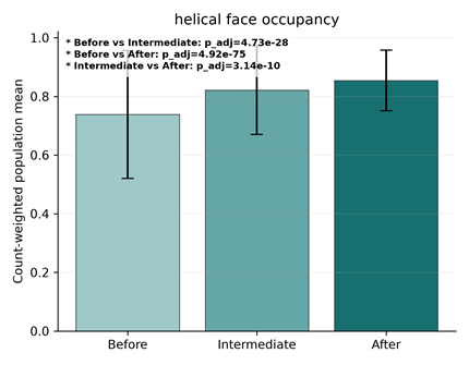
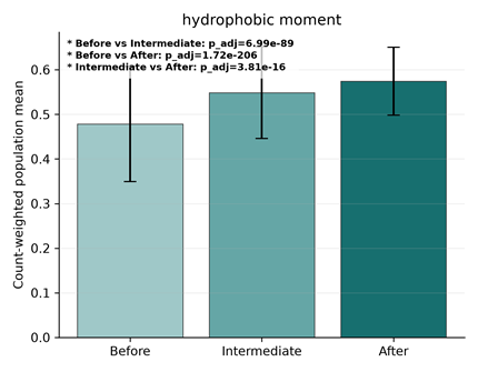
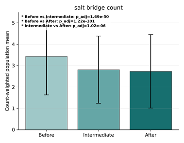
Figure 3. Comparison of helical face occupancy, hydrophobic moment and salt bridge counts of CAHS1 derived library at o rounds (Before), 3 rounds (Intermediate) and 6 rounds (After) of freeze-thaw selection.. * Indicates statistical significance by Mann-Whitney U Test.
Clustering was performed on sequencing data for samples that had gone through 0, 3 and 6 freeze thaw cycles. Across selection rounds, decreases in Pace-Scholtz sums and means as well as increase in helical face occupancy were observed. The cluster maps and traits within each cluster are shown below.
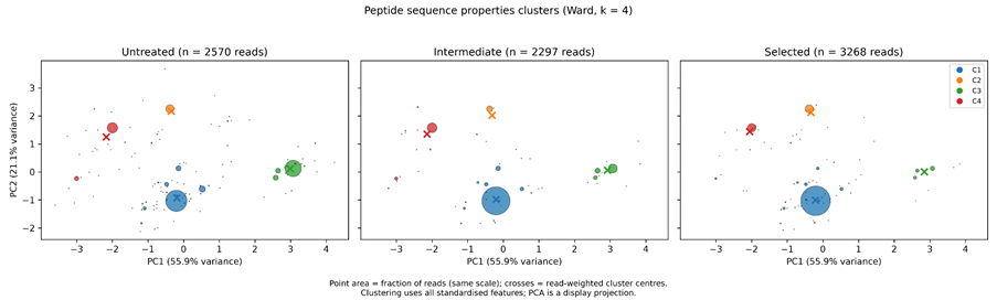
Figure 5. Cluster diagrams of CAHS1-derived libraries at 0 (untreated), 3 (intermediate) and 6 (selected) rounds of freeze-thaw selection.
Table 4. Proportional population size of different clusters in the library of CAHS before, during, and after selection.
| C1 proportion | C2 proportion | C3 proportion | C4 proportion | |
|---|---|---|---|---|
| Round 0 | 51.9% | 6.38% | 29.6% | 12.1% |
| Round 3 | 75.6% | 3.48% | 10.9% | 10.0% |
| Round 6 | 82.7% | 6.43% | 3.79% | 7.04% |
In the current four-cluster representation (mean silhouette score = 0.367), the increased representation of C1 was accompanied by decreased representation of C3 and C4. The read-weighted within-cluster PCA centres remained comparatively similar, indicating that substantial changes in variant frequencies were accompanied by smaller changes in the average properties represented by the first two principal components.
The dominant variant identified by enrichment in C1, CAHS1-055, increased from 1,027 of 2,570 reads (40.0%) in the round 0 sample to 2,509 of 3,268 reads (76.8%) after round 6. This represented an approximately 1.92-fold increase in relative abundance.
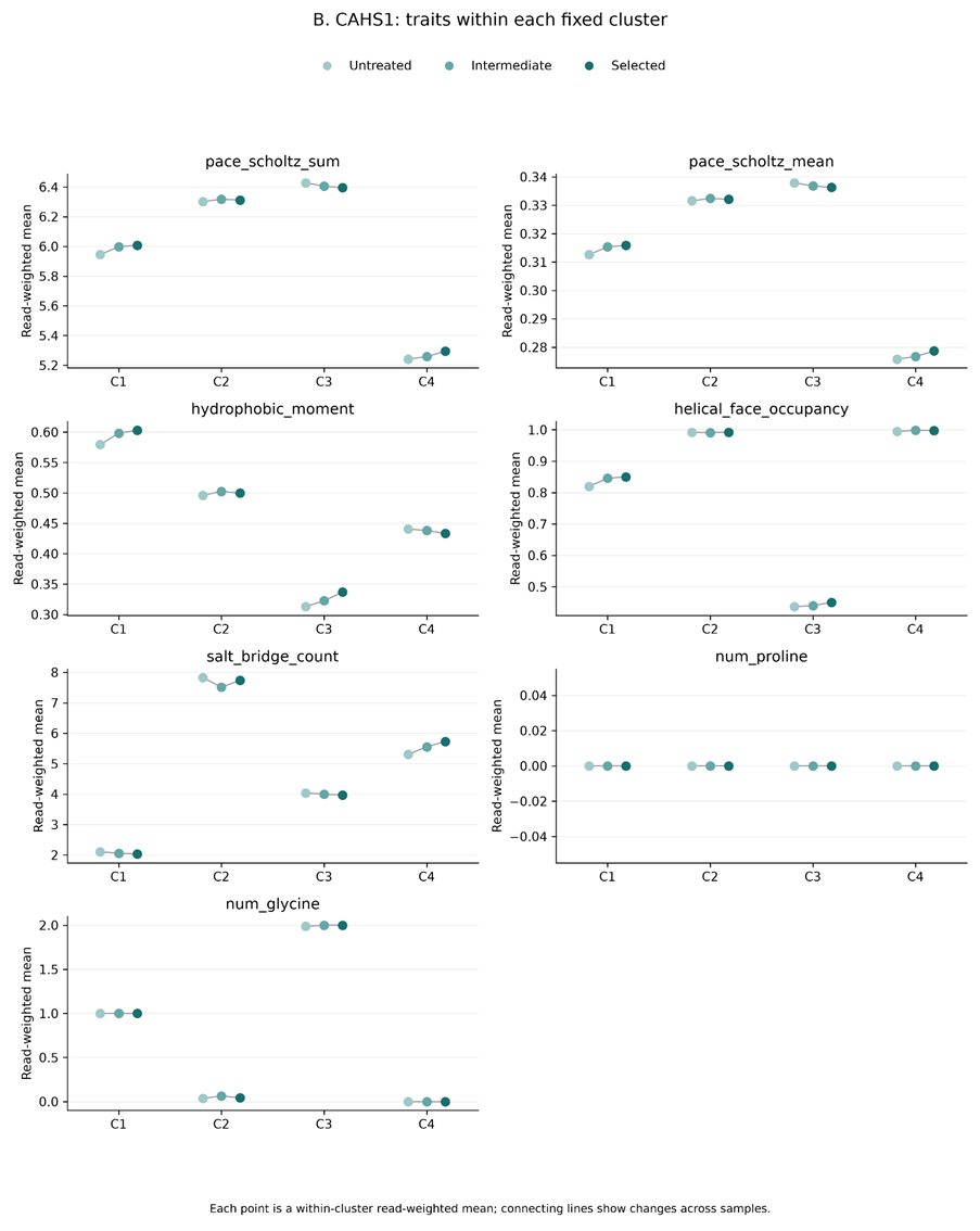
Figure 6. Comparison of read-weighted means of CAHS1 related properties between clusters before and after selection.
Post selection, C1 displayed intermediate values of read-weighted mean Pace-Scholtz sum (6.01) and mean (0.316). C1 displayed the lowest read-weighted mean salt bridge count (2.03) compared to C3 (3.97) and C4 (5.73).
C2 counts for the lowest representation among all clusters and displayed no significant change in percentage representation within the population across all 3 rounds and displayed the highest salt bridge count post selection (7.73).
Discussions:
For CAHS1, the current analysis illustrates how substantial sequence-level redistribution can coexist with comparatively stable within-cluster PCA centres: variants can differ in abundance while occupying similar regions of the measured property space.
Comparison between variants:
Winner sequence (motif 1 only): IRRQMRRAKGRIRKEMTKM
| Pace–Scholtz sum | Pace–Scholtz mean | Hydrophobic moment | Helical face occupancy | Salt bridge count | Number of proline | Number of Glycine | Helix breaker flag |
|---|---|---|---|---|---|---|---|
| 6.03 | 0.317 | 0.609 | 0.857 | 2 | 0 | 1 | True |
Original CAHS Core sequence (motif 1 only): YRKQQEVEADKIRKELEKQ
| Pace–Scholtz sum | Pace–Scholtz mean | Hydrophobic moment | Helical face occupancy | Salt bridge count | Number of Proline | Number of Glycine | Helix breaker flag |
|---|---|---|---|---|---|---|---|
| 6.68 | 0.352 | 0.263 | 0.6 | 9 | 0 | 0 | FALSE |
Worst performing (motif 1 only): RRKRMGKEKGRVRKELAKM
| Pace–Scholtz sum | Pace–Scholtz mean | Hydrophobic moment | Helical face occupancy | Salt bridge count | Number of Proline | Number of Glycine | Helix breaker flag |
|---|---|---|---|---|---|---|---|
| 6.45 | 0.339 | 0.304 | 0.429 | 4 | 0 | 2 | True |
Decrease in salt bridge count
From statistical analysis, it is shown that on a population level, the salt-bridge count decreases, and on a cluster-level, C1 has the lowest salt-bridge count while being the most enriched.
The salt bridge count is a sequence-based proxy: the number of oppositely charged residue pairs at i→i+3 or i→ i+4 spacing, which could form helix-compatible ion pairs. Those spacings put side chains on the same face of an alpha-helix (3.6 residues per turn). It counts every acidic/basic residue pair separated by 3 or 4 positions. It does not establish that such interactions will occur, how tight the interactions are or account for the pH of the environment.
Schematic representation of salt bridge count:
Side View of Helix Wall
—[ i ]— (e.g., Glutamate - negative charge)
|(Salt Bridge)
|—[ i+3 ]— (e.g., Lysine - positive charge)
The decline in this count after selection was driven mainly by the depletion of acidic residues (glutamic acid, aspartic acid). Nevertheless, the pairs per acidic residue were similar across the wild type, winner and the worst performing variants.
However, because the winner’s helical signal stayed high despite losing most pairs, we hypothesise that its helical propensity comes from other residues and does not depend on ion pairs. Future work to investigate this property can involve restoring glutamic acid or aspartic acid residues in the winner at i + 4 from a lysine or arginine residue and compare the helicity by circular dichroism.
These results suggest that this allows for greater flexibility or fewer charge-mediated intermolecular contacts that promote aggregation.
Face Occupancy, Hydrophobic Moment and Pace-Scholtz Sums and Means
From the scores between the winner variant and the worst performing variant, alongside the result from the analysis of the sequencing data, it can be seen that there is a:
1.  Increase in face occupancy

2.  Increase in hydrophobic moment

3.  Decrease in Pace-Scholtz sums and means
This suggests that selection favoured variants with hydrophobic residues more concentrated on one face with a stronger amphipathic helical character.
This is consistent with Kang et al’s observations of CAHS1 motif 1 being an amphipathic alpha-helix (Kang et al, 2024).
As to why this is important in protecting E.coli from freeze-thaw, we hypothesise that it is because an amphipathic helix can protect membranes during freezing. From Tolleter et al., 2010, the leakage experiments show that the pea mitochondrial LEA protein LEAM, which also forms an amphipathic alpha helix, stabilises liposomes under both drying-rehydration and freeze-thaw. Protection was greater with mitochondria-mimicking lipid mixtures, particularly those containing cardiolipin, than with pure POPC. The authors proposed that LEAM folds into an amphipathic alpha-helix on drying and interacts electrostatically with phospholipid headgroups, based on spectroscopic data and a structural model. They also suggested that similar interactions can probably occur with phosphatidylethanolamine (PE). E.coli’s membrane contains 76 to 77% PE (Shokri and Larsson, 2004). These experiments used liposomes of defined composition, not living cells, and the strongest protection was seen with cardiolipin-rich mitochondrial-like lipid mixtures. E.coli membranes are PE-dominant and contain less cardiolipin, so whether similar protection would occur is untested here.
Additional information on hydrophobic moment and helical face occupancy
What do hydrophobic moment and helical face occupancy mean?
Each residue contributes a vector whose magnitude is its hydrophobicity and whose direction corresponds to its position around the helix. Summing these vectors gives the hydrophobic moment; the direction of the resulting vector indicates the predominant hydrophobic direction, while its magnitude indicates the strength of the directional hydrophobicity. Therefore, it provides a direction corresponding to the predominant directional distribution of hydrophobicity around the alpha-helix. A 120° sector (± 60° from this direction) was therefore defined as the hydrophobic face.
Face occupancy was calculated as the fraction of residues with positive hydrophobicity (h > 0) that fell within this sector. Higher values indicate greater concentration of hydrophobic residues within the hydrophobic-moment-defined-face. Because this metric considers only whether the residues exceed the hydrophobicity threshold, it measures the spatial concentration of hydrophobic residues rather than their hydrophobicity or the hydrophilicity of the opposing face.
CALVADOS Simulations
Details of the parameters calculated:
Fraction of non-monomeric chains (non_mono_mp1, non_mono_mp5, non_mono_mp10):
The fraction of chains that belong to a cluster containing at least two chains. Two residues from different chains are considered to be in contact when their distance is ≤ 0.7nm. For mp=1, two chains were considered connected if they had at least one inter-chain residue-residue contact. For mp=5, two chains were only considered connected if they had at least 5 inter-chain residue-residue contacts. For mp=10, two chains were only considered connected if they had at least 10 inter-chain residue-residue contacts. Non_mono_mp1, non_mono_mp5, and non_mono_mp10 were calculated as the fraction of all chains belonging to clusters of size ≥2. Higher values therefore indicate that a greater proportion of chains participate in inter-chain associations.
Contacts/chain:
the number of residues per chain that are in contact with other residues in an inter-chain association
Largest cluster fraction:
largest cluster size / 20, i.e. how big the biggest cluster is out of 20 chains.
Mean Rg:
shows how compact the variants are
Analysis
Fraction of non-monomeric chains
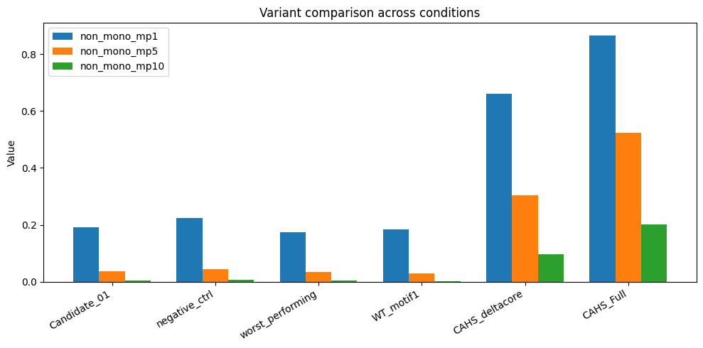
Figure 7. Fraction of non-monomeric chains in the CALVADOS simulations.
Note:
WT_motif1: original CAHS Core with motif 1
Negative_ctrl: the randomly shuffled WT_motif1
Candidate_01: Winning sequence
Worst_performing: the least enriched sequence
Dashed = CAHS Core with motif 1’s result
Error bars = block SEM within one run (omitted for non-monomeric fraction; values in the notebook results table:CALVADOS For CAHS)
n = 1 run each
| variant | non_mono_mp1 | non_mono_mp5 | non_mono_mp10 |
|---|---|---|---|
| Candidate_01 | 0.192 | 0.038 | 0.005 |
| negative_ctrl | 0.225 | 0.045 | 0.006 |
| worst_performing | 0.174 | 0.034 | 0.004 |
| WT_motif1 | 0.184 | 0.030 | 0.003 |
| CAHS_deltacore | 0.660 | 0.305 | 0.096 |
| CAHS_Full | 0.866 | 0.524 | 0.202 |
From the table and bar graph, it can be seen that the fraction of non-monomeric chains of CAHS Full is the highest at every threshold, followed by ΔCore. At mp =1, about 87% of CAHS Full chains (~17 of 20) were in a cluster, falling to about 20% (~4 chains out of 20) at mp=10, which indicates that a substantial part of its association is by looser contacts. This also suggests that it is more prone to associating with each other. ΔCore showed an intermediate level (66 % at mp = 1, 10% at mp = 10).
In contrast, at mp = 1, only around 17-23% of chains (~4 chains out of 20) form part of a cluster for the negative control, CAHS Core, the winning sequence and the worst performing variant and essentially none at mp=10. Most chains therefore remain as monomers, which is in line with the lack of aggregation reported for CAHS Core by Kang et al. This shows that the evolved variants, to a certain extent, still share the intrinsic baseline property of CAHS Core as neither selected variant showed a detectable increase in self-association relative to CAHS Core and the simulations reproduced the Full > ΔCore > Core ordering in terms of their ability to self-associate. However, as these are single runs, small differences between the Core-length sequences are not resolved.
Contacts/chain
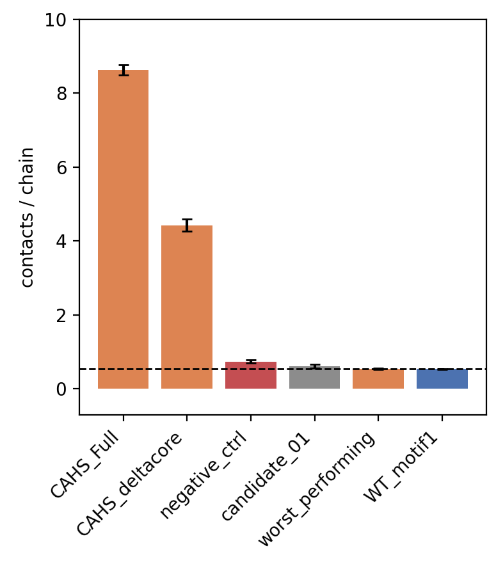
Figure 7. Contacts per chain in the CALVADOS simulations.
As shown in the graph, it can be seen that the contacts per chain for CAHS Full and is the highest, followed by CAHS ΔCore, with the negative control, winning variant, worst performing variant and CAHS Core having the least number of contacts per chain.
This is consistent with the above result that indicates that CAHS Full and CAHS ΔCore have more residues in contact with one another, further showcasing their aggregation-prone nature.
Largest cluster fraction
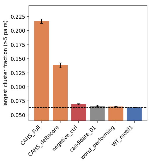
Figure 8. Largest cluster fraction at the five-contact threshold.*
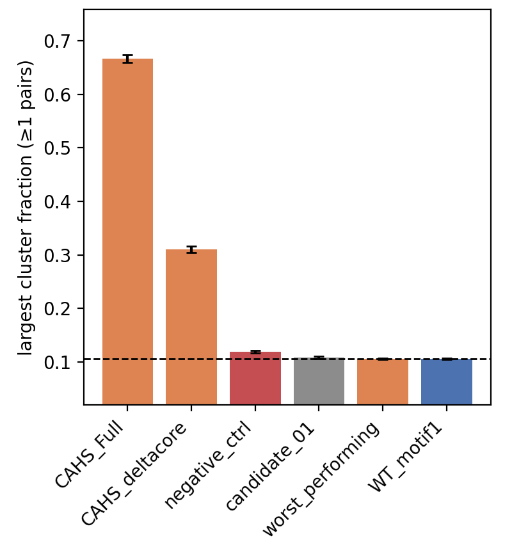
Figure 9. Largest cluster fraction at the one-contact threshold.
The largest cluster fraction is the number of chains out of 20 chains that exists in the largest cluster formed by the chains. As shown in the figures, in the case where the chains are considered connected if they have at least 1 inter-chain residue-residue contact, CAHS Full has the largest cluster fraction of approximately 0.65, which suggests that approximately 13 chains form the largest cluster. CAHS ΔCore, on the other hand, has around 6 chains in the largest cluster. The negative control, winning variant, worst-performing variant and CAHS Core have only around 2 chains in the largest cluster, which indicates that most chains remain monomeric or dimeric at most. This also supports the results above, where CAHS Full chains seem to be loosely connected with one another and self-associate.
Therefore, as an in silico sanity check, CALVADOS simulations at 2 mM (293K, 0.09 M ionic strength) showed no detectable increase in intrinsic self-association for the winning variant relative to the original CAHS Core with motif 1, while the aggregation-prone ΔCore and Full constructs showed markedly higher clustering.
These results are therefore consistent with Kang et al’s findings, that is, the turbidity of CAHS Full and ΔCore rose with protein concentration, while CAHS Core stayed flat. They have also mentioned that their results suggest that the aggregation- or phase-separation-promoting regions are located at both N- and C- terminals, rather than at the Core.
Radius of gyration
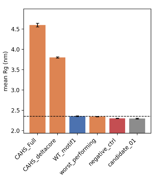
Figure 9. Mean radius of gyration in the CALVADOS simulations.
The mean per-chain Rg is around 2.3 to 2.4 nm for all the 63-residue sequences, including the winning variant, and increased with chain length to 3.80 nm for ΔCore and 4.60 nm for Full, consistent with an expanded, disordered ensemble. We hypothesise that this is because the per-chain Rg increases with the chain length, where Rg scales as a power law in the number of residues (Kohn et al., 2004). The evolved variants therefore retain the wild-type-like chain dimensions. Small differences among the Core-length sequences were not interpreted or analysed given the single-run design.
References
Bülow, S. von et al. (2025) ‘Software package for simulations using the coarse-grained CALVADOS model’. arXiv. Available at: [https://doi.org/10.48550/arXiv.2504.10408].
Kang, D. et al. (2024) ‘Protective roles of highly conserved motif 1 in tardigrade cytosolic-abundant heat soluble protein in extreme environments’, Protein Science, 33(3), p. e4913. Available at: [https://doi.org/10.1002/pro.4913].
Kohn, J.E. et al. (2004) ‘Random-coil behavior and the dimensions of chemically unfolded proteins’, Proceedings of the National Academy of Sciences of the United States of America, 101(34), pp. 12491–12496. Available at: [https://doi.org/10.1073/pnas.0403643101].
Nick Pace, C. and Martin Scholtz, J. (1998) ‘A Helix Propensity Scale Based on Experimental Studies of Peptides and Proteins’, Biophysical Journal, 75(1), pp. 422–427. Available at: [https://doi.org/10.1016/S0006-3495(98)77529-0].
Shokri, A. and Larsson, G. (2004) ‘Characterisation of the Escherichia coli membrane structure and function during fedbatch cultivation’, Microbial Cell Factories, 3, p. 9. Available at: [https://doi.org/10.1186/1475-2859-3-9].
Sleight, S.C., Wigginton, N.S. and Lenski, R.E. (2006) ‘Increased susceptibility to repeated freeze-thaw cycles in Escherichia coli following long-term evolution in a benign environment’, BMC Evolutionary Biology, 6(1), p. 104. Available at: [https://doi.org/10.1186/1471-2148-6-104].
Tolleter, D., Hincha, D.K. and Macherel, D. (2010) ‘A mitochondrial late embryogenesis abundant protein stabilizes model membranes in the dry state’, Biochimica et Biophysica Acta (BBA) - Biomembranes, 1798(10), pp. 1926–1933. Available at: [https://doi.org/10.1016/j.bbamem.2010.06.029].
Zhang, J. et al. (2025) ‘Rationally designed highly amphipathic antimicrobial peptides demonstrating superior bacterial selectivity relative to the corresponding α-helix peptide’, European Journal of Medicinal Chemistry, 286, p. 117310. Available at: [https://doi.org/10.1016/j.ejmech.2025.117310].