Principle

RFDiffusion is a cutting-edge method for de novo protein structure and function design, leveraging the capabilities of deep learning and diffusion models. It is based on the RoseTTAFold (RF) structure prediction network, fine-tuned on protein structure denoising tasks. The principle behind RFDiffusion is to generate protein backbones by iteratively refining noise-corrupted structures, eventually producing functional and structurally accurate proteins from simple molecular specifications.

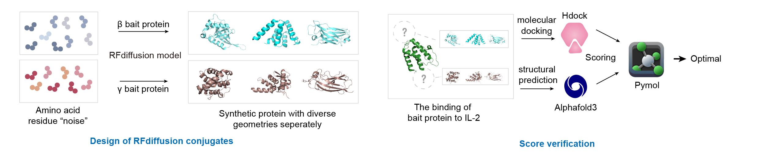
HDOCK server is a free docking framework based on hybrid docking strategy, which automatically incorporate the binding interface information into traditional global docking, and realize the sampling and scoring of protein and protein docking with robustness and high speed. Although developers claim that HDOCK can realize the docking between protein and nucleic acid, it is still difficult because of the complexity and flexibility of nucleic acid structure. HDOCK server integrates homology search, template-based modeling, structure prediction, global docking, biological information integration and job management, and supports downloading and visual interaction, so it is friendly to non-professional biologist.

AlphaFold3 is a state-of-the-art protein structure prediction tool developed by DeepMind. It utilizes deep learning techniques to quickly and accurately predict the three-dimensional structure of proteins based on their amino acid sequences. This advanced AI system has significantly improved the speed and accuracy of protein structure predictions, making it a valuable resource for biological research, drug discovery, and understanding the functions of proteins in the body. AlphaFold3 builds upon the success of its predecessors, offering a more efficient and reliable way to predict protein structures, which can aid in the development of new therapeutics and deepen our understanding of biological systems.

Method

A. RFDiffusion

1. Model Training

① Data Preparation: Sample protein structures from the Protein Data Bank (PDB) and introduce noise to create training inputs.

② Noise Application: Perturb Cα coordinates with 3D Gaussian noise and apply Brownian motion to residue orientations.

③ Model Training: Train the RFDiffusion model by minimizing the mean-squared error (MSE) loss between frame predictions and the true protein structure.

2. Protein Design

① Initialization: Start with random residue frames.

② Denoising Iterations: Iteratively refine the protein structure by denoising the noisy input, adding noise at each step to generate the input for the next iteration.

③ Sequence Design: Use the ProteinMPNN network to design sequences encoding the generated protein structures.

3. Conditioning for Specific Designs

① Unconditional Design: Generate diverse protein structures without additional input.

② Topology-Constrained Design: Provide secondary structure and/or fold information to guide the design towards specific topologies.

③ Symmetric Oligomer Design: Specify point group symmetry to create symmetric oligomeric structures.

4. Experimental Characterization

① Expression and Purification: Express the designed proteins in a suitable host and purify them for further analysis.

② Structural Verification: Use techniques such as circular dichroism (CD) and cryo-electron microscopy (cryo-EM) to verify the structure and stability of the designed proteins.

③ Functional Validation: Assess the functionality of the designed proteins through binding assays, enzymatic activity tests, or other relevant functional assays.

B. HDOCK

1. Data input

The HDOCK web server is available at http://hdock.phys.hust.edu.cn/. Both sequence and structure information of ligand and receptor should be uploaded through the website separately. The docking process will be carried out in the server. Click submit to wait for the results. Generally, the waiting time is approximately 30 minutes. The submitted sequences should be in FASTA format and contain only standard amino acids. The structure should be in PDB format. In addition, residue information of the binding sitei is also possible to be submitted as a filter in the docking process.

2. Docking preparation

First, the homologous sequences of molecules will be searched by sequence similarity search. The template with the highest sequence coverage, highest sequence similarity and highest resolution will be selected to build the template-based model. ClustalW is used for sequence alignment, and MODELLER is used for model construction. This step will be executed on the server.

3. Global docking

HDOCKlite, a layered docking program based on FFT, is used to globally sample the presumed binding directions. If the binding site information was provided when submitting, the docking process will also include it. The ranked binding modes are clustered with an RMSD cutoff of 5 Å. if two binding modes have a ligand RMSD of ≤ 5 Å, the one with the better score is kept. This step will be executed on the server. The docking model of HDOCKlite and the template-based docking model of MODELLER will be provided for download through web interaction.

4. Results analysis

The server will send the top 10 docking models to the website. The results page contains an interactive visualization window and a summary table. The summary table usually contains docking energy score, confidence score and ligand RMSD. If the SAXS data file is provided, the SAXS chi-square of the model can also be displayed. Results can also be downloaded as a PDB file, using the molecular visualization software PyMOL to open and view the predicted model.

C. AlphaFold3

1. Data Retrieval

① Retrieve Template Structures: The model retrieves template structures from PDBmmCIF files. This involves parsing the files to extract the relevant structural information that can serve as a template for the prediction of the target protein structure.

② Database Sequence Retrieval: Retrieve protein sequences from five databases to be used for multiple sequence alignment (MSA). And retrieve RNA sequences from three databases, also for MSA purposes. These sequences help in understanding the evolutionary context and the potential interactions with the protein of interest.

2. Sequence and Token Processing

① Tokenization: Convert the input sequences (protein and RNA), ligands, and covalent bonds into tokens. Tokenization is the process of breaking the sequences into smaller units that can be processed by the neural network.

② Embedding: Input the tokens into an embedder, which is a component of the neural network designed to convert tokens into high-dimensional vectors (embeddings) that capture their meaning in the context of the model. The embedder will output three types of embeddings:

Input Embeddings: Representations of the input sequences.

Single Embeddings: Representations of individual tokens.

Pair Embeddings: Representations of pairs of tokens, which capture the relationships between different parts of the sequences.

3. Structure Generation and Refinement

① Integration of Information: Combine the template structure information with the pair embeddings obtained from the feature extraction module. Integrate MSA information to generate a pair representation that captures the evolutionary and structural relationships within the sequences.

② Representation Regulation: Use the Pairformer module to organize and update the single representation and pair representation information. This module ensures that the relationships between different parts of the protein are accurately reflected in the model’ representations. And the single and pair representations are updated iteratively through multiple cycles to refine and improve their accuracy.

③ Structure Prediction: Pass the encoded information through a diffusion model, which progressively adds noise to the data and then denoises it to generate a clear three-dimensional structure of the protein. Then use metrics such as pLDDT (predicted local distance difference testing), PAE (predicted alignment error), and PDE (predicted distance error) to assess the confidence of the predicted structure. These metrics provide insight into the quality and reliability of the predicted protein structure.

Principle

ClonExpress technology is a simple, fast and efficient technique for seamless DNA cloning, allowing targeted cloning of insert fragments into any site of any vector. The vector is linearized by introducing the terminal sequence of the linearized vector at the 5’ end of the forward/reverse PCR primer of the insert, so that the 5’ and 3’ ends of the PCR product have the same sequence (15 - 20 bp) as the two ends of the linearized vector, respectively. After the PCR product and linearized vector were mixed in a certain proportion, the reaction can be carried out at 37℃ for 30 min under the catalysis of recombinase to complete the targeted cloning.

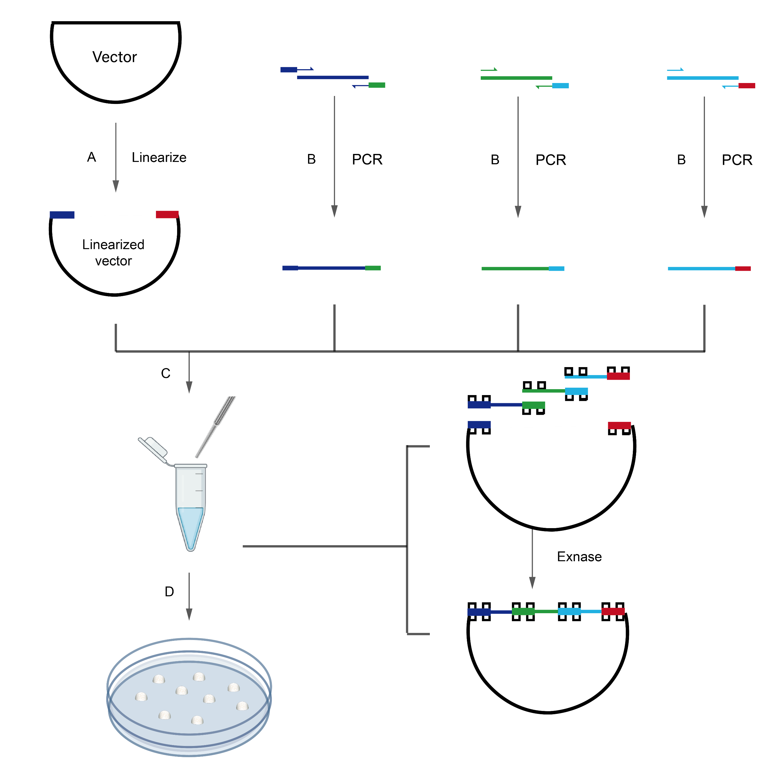
A. Vector linearization: The linearized vector was obtained via restriction enzyme digestion or inverse PCR.

B. Insert fragment acquisition: Homologous sequences corresponding to the 15-20 bp terminal regions of the linearized vector were added to the 5’ ends of the gene-specific forward/reverse amplification primers. The insert fragment containing homologous arms was amplified using these primers.

C. Recombination reaction: The linearized vector and insert fragment were mixed at an optimal ratio, followed by a 5-30 minutes recombination reaction catalyzed by Exnase (2×CE Mix) at 50°C to achieve in vitro circularization of the multiple linear DNA fragments.

D. Transformation of competent cells: The recombinant products were directly transformed into competent cells, yielding hundreds of single colonies on agar plates for subsequent positive screening.

Method

A. Preparation of Linearized Vector

1. Suitable cloning sites are chosen for vector linearization. Sites lacking repetitive sequences and exhibiting GC content between 40% and 60% within the 20 bp regions upstream and downstream of the cloning site are preferentially selected.

2. The vector can be linearized via restriction enzyme digestion or inverse PCR amplification.

B. Acquisition of Insert Fragment

1. General primer design principles: Homologous sequences corresponding to the termini of the linearized vector are introduced at the 5’-ends of the forward and reverse amplification primers for the insert fragment. This ensures that the amplified insert fragment contains terminal homologous sequences at its 5’ and 3’ ends that match the corresponding sequences of the linearized vector. Forward primer design: 5’–[Homologous sequence from upstream vector terminus] + [Restriction site (retained or removed)] + [Gene-specific forward primer sequence]–3’. Reverse primer design: 5’–[Homologous sequence from downstream vector terminus] + [Restriction site (retained or removed)] + [Gene-specific reverse primer sequence]–3’.

2. PCR amplification of insert fragment: The insert fragment is amplified using any PCR polymerase, with no requirement to consider the presence or absence of A-overhangs at the product termini.

C. Quantification of Linearized Vector and Insert Fragment

1. Concentration determination: DNA quantification is recommended to be performed via electrophoresis with band intensity comparison, as specified for the ClonExpress homologous recombination system.

2. Calculation of vector fragment usage: The optimal amount of linearized vector for the ClonExpress II recombination system is 0.03 pmol, while the optimal insert fragment amount is 0.06 pmol (molar ratio of vector to insert = 1:2).

The corresponding DNA mass can be approximated using the following formulas:

Optimal vector usage = [0.02 × vector base pairs] ng (equivalent to 0.03 pmol).

Optimal insert usage = [0.04 × insert base pairs] ng (equivalent to 0.06 pmol).

D. Recombination Reaction

1. The required amounts of DNA for the recombination reaction are calculated based on the formulas provided above. To ensure pipetting accuracy, the linearized vector and insert fragment may be appropriately diluted prior to assembling the recombination reaction system. The volume of each component added should not be less than 1 μl.

2. The following reaction system is prepared on ice:

Group	Linearized Vector (μl)	Insert Fragment (μl)	2×CE Mix (μl)	ddH2O (μl)
Recombination	X	Y	5	to 20
Negative Control-1	X	0	0	to 20
Negative Control-2	0	Y	0	to 20
Positive Control	1	0	5	to 20

3. The reaction mixture is gently mixed by pipetting (vortexing is avoided), followed by brief centrifugation to collect the liquid at the bottom of the tube.

4. The reaction is incubated at 37°C for 30 min, then cooled to 4°C or immediately placed on ice.

E. Transformation Procedure

1. Cloning-competent cells are thawed on ice.

2. 10 μl of the recombination product is added to 100 μl of competent cells. The mixture is gently mixed by flicking the tube (vortexing is avoided) and incubated on ice for 30 min.

3. Cells are heat-shocked in a 42°C water bath for 45 sec, then immediately transferred to ice for 2–3 min.

4. 900 μl of SOC or LB medium is added, followed by incubation at 37°C with shaking (200–250 rpm) for 1 h.

5. LB agar plates containing the appropriate antibiotic are pre-warmed in a 37°C incubator.

6. The culture is centrifuged at 2,400 × g for 5 min, and 900 μl of supernatant is discarded. The pellet is resuspended in the remaining medium and evenly spread onto the pre-warmed antibiotic-containing plates using a sterile spreading rod.

7. Plates are inverted and incubated at 37°C for 12–16 h.

F. Verification of Recombinant Products

1. Colony observation: After overnight incubation, hundreds of single colonies are observed on the recombinant product transformation plate, while significantly fewer colonies are present on the negative control plate.

2. Colony PCR screening: Several colonies from the recombinant plate are selected for colony PCR. At least one universal sequencing primer from the vector is used for amplification. A band slightly larger than the insert fragment size is expected if the clone is correct.

3. Further validation: PCR-positive colonies are inoculated into liquid LB medium containing the appropriate antibiotic and cultured overnight. Plasmid DNA is extracted for restriction enzyme digestion analysis or directly subjected to Sanger sequencing.

Principle

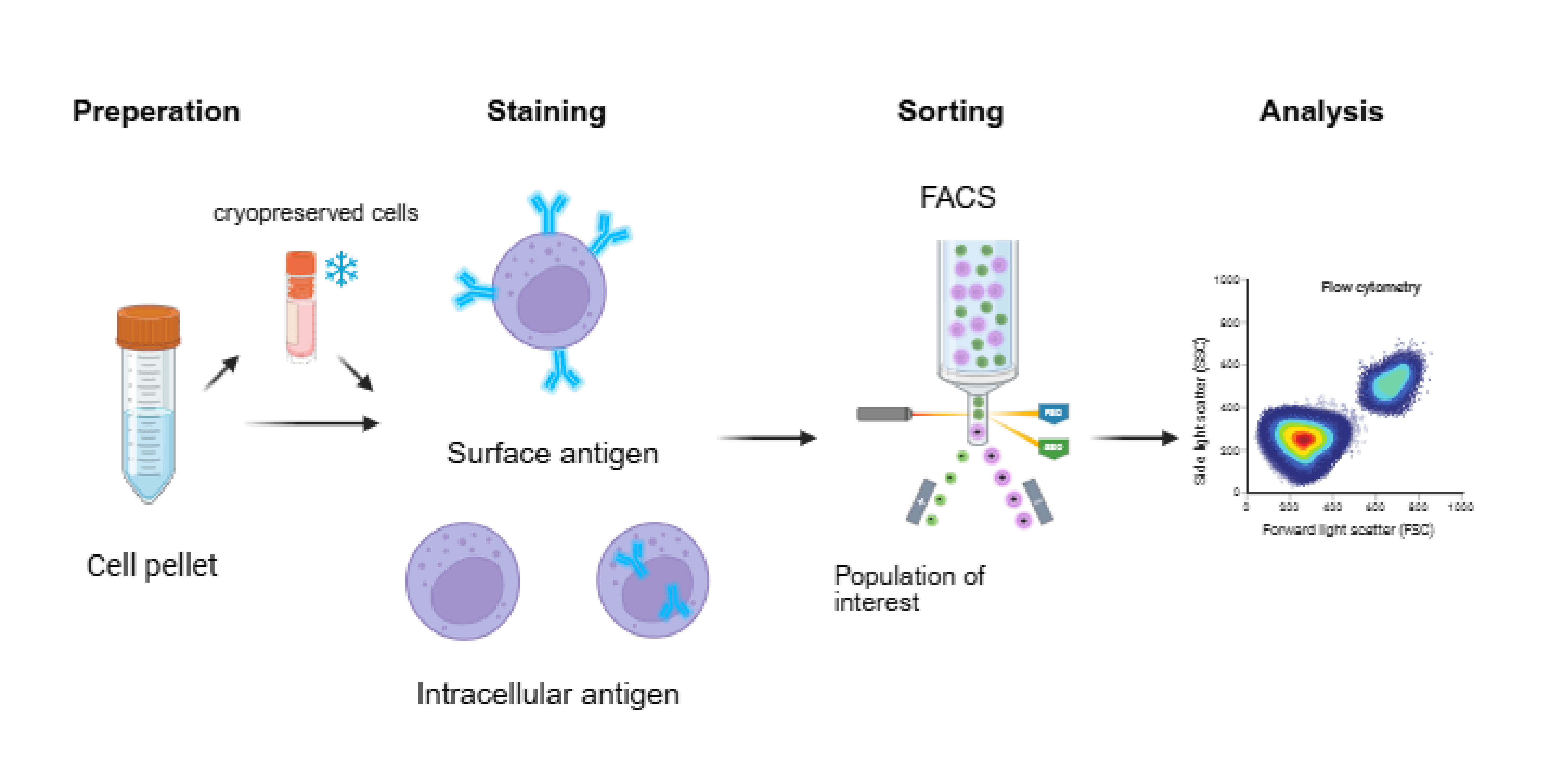
Perforin (PFN) and granzyme (GrB) are key effector molecules for natural killer (NK) cell cytotoxicity, stored within cytoplasmic granules. In this experiment, their secretion was inhibited using the protein transport inhibitor Brefeldin A, causing intracellular accumulation. Following fixation and membrane disruption, fluorescent antibodies were introduced to bind specifically to these molecules within the cells, enabling quantitative detection via flow cytometry.

Method

A. Cell resuscitation

1. Co-culture target cells (K562) in logarithmic growth phase with effector cells.

2. (pre-stimulated NK cells) at a specific effector-to-target ratio in a 37°C, 5% CO₂ incubator.

3. Add Brefeldin A (diluted 1:1000) to the co-culture system 12 hours after initiation. Continue culture for a total of 46 hours.

4. After co-culture, collect cells into flow cytometry tubes. Wash once with pre-chilled PBS, centrifuge at 300 × g for 5 minutes, and discard the supernatant.

5. Resuspend cells in 100 μL flow cytometry staining buffer for cell counting.

B. Surface Staining

1. Dosage example for a 100 μL reaction system:CD3-PerCPCy5.5 (1:1000), CD56-PE (1: 1000).

2. Add antibodies to the cell tube, gently mix by pipetting, and incubate at 4°C in the dark for 30 minutes.

3. Wash with 2 mL staining buffer, centrifuge at 300 × g for 5 minutes, discard supernatant. Repeat washing once.

C. Fixation and Membrane Permeabilization

1. Resuspend cells in 100 μL fixative, incubate at room temperature in the dark for 15-20 minutes.

2. Add 2 mL staining buffer, centrifuge, discard supernatant, and thoroughly remove fixative.

3. Resuspend cells in 100 μL lysis buffer and incubate at room temperature in the dark for 15-20 minutes.

D. Intracellular Staining

1. Dilute intracellular antibodies in lysis buffer: Perforin-FITC (1:1000), Granzyme-BB421 (1: 1000), Centrifuge and discard lysis buffer.

2. Add the intracellular antibody cocktail to the cell tube, gently pipette to mix, and incubate at room temperature in the dark for 30-45 minutes.

3. Wash with 2 mL lysis buffer, centrifuge at 300 × g for 5 minutes, and discard the supernatant. Repeat the wash once.

4. Resuspend cells in 300-500 μL flow cytometry staining buffer and analyze immediately.

E. Data Analysis:

1. The suspension was transferred to flow cytometry sample tubes.

2. Analysis Strategy:

(1) Gate to exclude doublets (using FSC-A vs FSC-H).

(2) Gate to exclude dead cells (using a viability dye).

(3) Identify the target cell population (NK cells: CD3⁻ CD56⁺).

(4) Analyze PFN and GrB expression: Percentage of positive cells (%) and MFI.

Principle

Bio-Layer Interferometry (BLI) is a label-free technology that converts the optical interference signals generated on the surface of a BLI biosensor into real-time response signals. By monitoring the molecular binding process in real time, the system measures the association constant (ka or kon), dissociation constant (kd or koff), and initial binding rate, and further derives affinity (KD) and concentration information through fitting and computational analysis.

Octet biosensors are constructed from glass optical fibers, with an additional specialized optical layer applied to the distal end. This optical layer provides a surface chemistry matrix for ligand immobilization. White light, encompassing all wavelengths within the visible spectrum, is introduced into the optical fiber and undergoes partial internal reflection at two interfaces: the interface between the glass fiber and the optical layer (which is fixed), and the interface between the surface chemistry and the solution (which is variable). The two beams of reflected light from these interfaces create an interference phenomenon. The instrument measures and records the intensity of the interfering light at each wavelength, generating an interference spectrum. Wavelengths that undergo constructive interference appear as peaks (high amplitude) on the spectrum, while those experiencing destructive interference appear as valleys (low amplitude). The Octet interaction analyzer detects molecular interactions by measuring changes in this interference spectrum in real time.

When molecules bind to the ligand immobilized on the biosensor surface, the thickness of the optical layer increases, resulting in a longer path length for the second reflected beam. This causes a shift in the interference spectrum towards longer wavelengths (a rightward shift). Conversely, when molecules dissociate from the ligand into the solution, the interference spectrum shifts back towards shorter wavelengths (a leftward shift). A plot of the shift in the interference spectrum (in nanometers) versus the time of the reaction is known as a Sensorgram. Based on the Sensorgram, the values of ka, kd, and KD can be determined by fitting the data to various binding models.

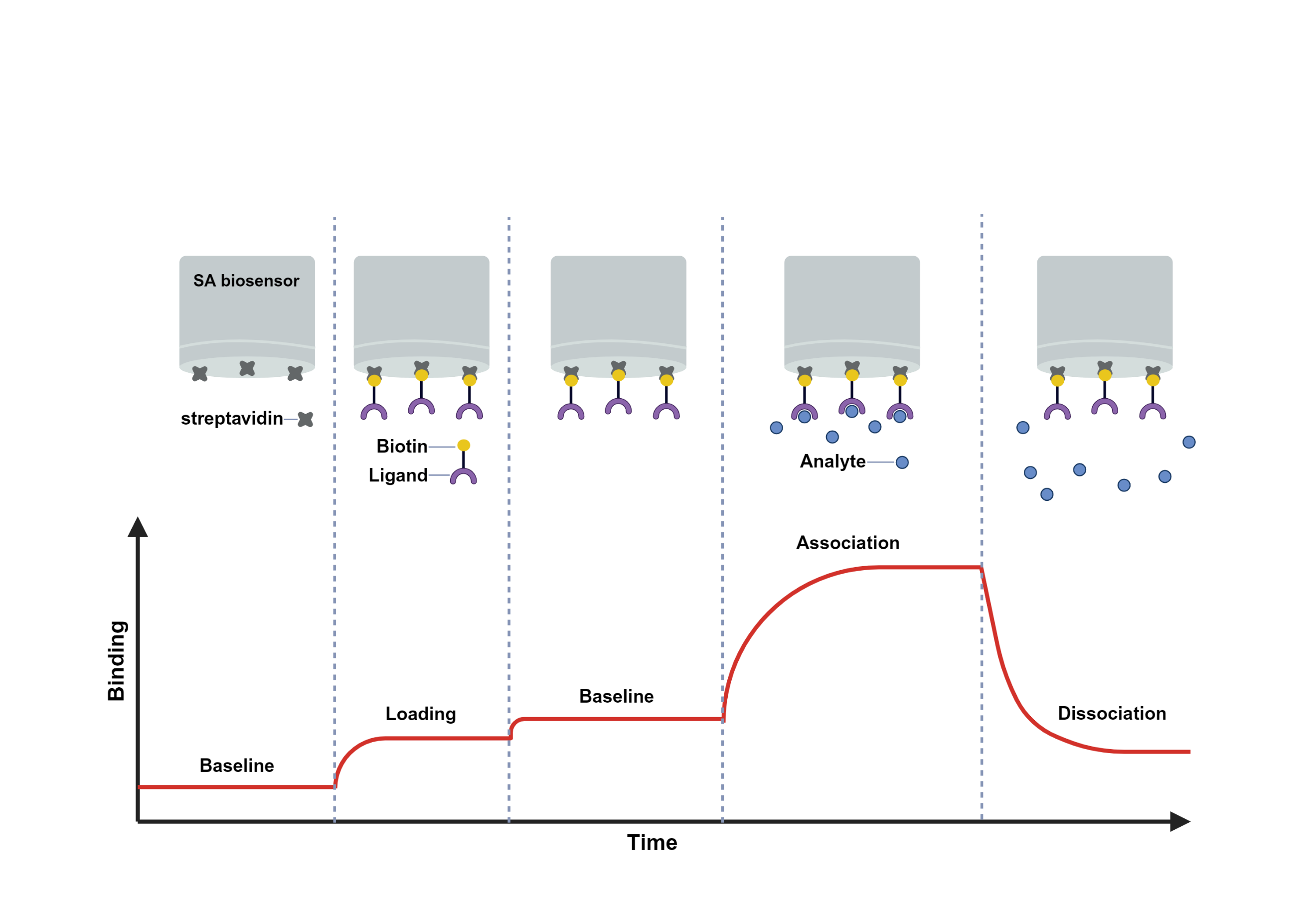
Fig. Experimental steps of biolayer interferometry.

Method

A. Sensor pre-humidification: Pre-wet plates were placed in a blue chassis (corner A1 of the sample plate needed to be snapped into the snap hole of the blue tray), and 200 μL of analytical buffer, such as PBST buffer and MES buffer, was added to the well where the sensor was placed. The sensor was placed on the green disk, and then the green disk was snapped onto the blue disk. The sensor needed to be pre-wetted for over 10 minutes.

B. Methods Edit: Within the Experiment Wizard software, the “New Kinetics Experiment-Basic Kinetics” option was selected. Following this, the protocol setup interface was accessed. The Basic Kinetics Experiment window was maximized, and the following five steps were sequentially edited:

1. Plate Definition: In the Plate Definition setup, four sample columns were designated as follows: Buffer1 was assigned to the baseline1 step, Load to the loading step, Buffer2 to both the baseline2 and dissociation steps, and Sample to the association step. The samples consisted of different test sequences at identical concentrations, with each well being loaded with 200 μg/L of the respective sample. Following the completion of parameter configuration, the experiment was initiated.

2. Assay definition: In the assay definition, the setup steps were followed by first clicking “Add” in the window to include the required analysis steps and set the duration for each one. The following steps were added: Baseline (60 s), Loading (120 s), Baseline2 (120 s), Association (180 s), and Dissociation (180 s), after which “OK” was clicked to confirm the selections. If any parameter required modification, it was edited by double-clicking. Next, in the “Step Data List,” the Baseline step was clicked, the arrow was moved to Baseline to indicate that the detection position for this step on the sample plate would be configured, and then the first column of samples on the sample plate was double-clicked, so that at the start of the experiment, the Baseline step would be detected using the samples in the first column (buffer). The “Assay Steps List” then displayed the first added step, showing that the Baseline analysis was performed using samples from the first column, with “No” indicating the step number, “Sample” representing the analysis location on the sample plate, and “Sensor Type” specifying the sensor selected for analysis. This process was repeated to complete the experimental setup for the entire kinetic analysis.

3. Sensor assignment: In the sensor assignment, the sensor position was configured.

4. Review Experiment: Clicking the buttons allowed browsing the previous or next step of the experiment respectively, enabling preview and verification of all experimental steps.

5. Run Experiment: After the setup was completed, the “Start Experiment” button was clicked. Before the experiment was initiated, it was ensured that the samples and sensors were properly placed and the instrument door was securely closed.

C. Result Analysis: The related data were acquired and processed using the data analysis software of the Octet system. Through this analysis, sensor grams were generated, from which kinetic parameters including KD, Kon, Koff, and steady-state fitting curves were derived. The consistency between the fitted and measured curves was evaluated. If the fitted curve showed strong agreement with the experimental curve, it indicated high quality of the fitting results. Based on these data, a comprehensive assessment of the binding affinity between the test sequences and the receptor was performed.

Principle

Molecular Dynamics (MD) refers to a computational simulation method used to study the physical movements of atoms and molecules over time, providing insights into their dynamic behavior at the atomic scale.

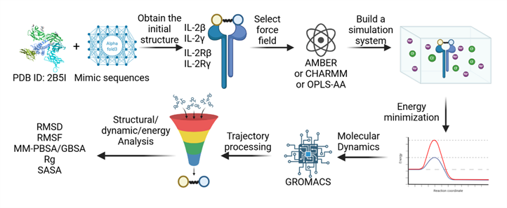
Figure 1. Work flow of Molecular dynamics simulation

Method

A. System Preparation

1. The receptor structure is modeled based on the X-ray crystal structure. The designed protein’s three-dimensional structure is predicted using AlphaFold3 and subjected to preliminary optimization.

2. Molecular docking is performed using HADDOCK software to obtain the initial binding structure of the receptor-protein complex. The structure with the lowest binding energy and optimal electrostatic interactions is selected as the initial conformation for subsequent molecular dynamics simulations.

3. The complex is placed in a periodic cubic water box, ensuring a minimum distance of 12 Å between any protein atom and the box boundary to provide sufficient solvation. The solvent environment is constructed using the TIP3P water model, with Na+ and Cl- ions added to neutralize the system and simulate physiological salt concentration.

4. The protein is parameterized using the CHARMM36m force field, the water molecules use the TIP3P model, and ion parameters are derived from the CHARMM force field.

B. Molecular Dynamics Simulation Settings

All molecular dynamics simulations are performed using the GROMACS 2022.5 software package.

1. Energy minimization is conducted using the steepest descent algorithm to eliminate unfavorable atomic contacts and geometric clashes.

2. In the first phase of equilibration (NVT), the system is equilibrated for 1 ns. Positional restraints with a force constant are applied to the protein backbone, allowing relaxation of the side chains and solvent molecules. In the second phase (NPT), the system is equilibrated with pressure controlled using the Berendsen pressure coupling method. During this phase, positional restraints on the solute are gradually reduced.

3. The production simulation is conducted in the NPT ensemble. The temperature is maintained using the velocity-rescaling thermostat, and the pressure is controlled using the Parrinello-Rahman pressure coupling method. Short-range interactions, including van der Waals and electrostatic forces, are calculated with a cutoff distance, while long-range electrostatics are computed using the particle mesh Ewald (PME) method with a grid spacing.

C. Data Analysis

1. GROMACS tools are used to analyze trajectory data, including calculations of root mean square deviation (RMSD), root mean square fluctuation (RMSF), and interaction changes at the binding interface residues.

2. Visual Molecular Dynamics (VMD) software is employed to visualize trajectories and extract snapshots for comparing the initial and final binding modes.

3. Fluctuations in van der Waals and electrostatic interactions are calculated and presented in radar charts to visually compare the binding performance of different complexes. B-factor analysis is integrated to evaluate the structural stability and residue fluctuations of the complex.

4. The initial and final binding interfaces are compared to analyze changes in key residue interactions.

Principle

The action of lactate dehydrogenase resulted in the reduction of NAD+ to form NADH. Subsequently, the combination of NADH and INT (2-p-iodophenyl-3-nitrophenyl tetrazolium chloride) was catalyzed by thioctylamine dehydrogenase (diaphorase) to form NAD+ and formazan. This process produced an absorption peak at 490 nm. Absorption peaks were generated at 490 nm, thus enabling the quantification of lactate dehydrogenase activity by colourimetry. Furthermore, the absorbance was found to be linearly and positively correlated with the activity of lactate dehydrogenase. Lactate dehydrogenase activity in cell lysates was assayed to evaluate the in vitro and ex vivo killing activity of NK cells. The schematic diagram of the principle is shown in Figure.

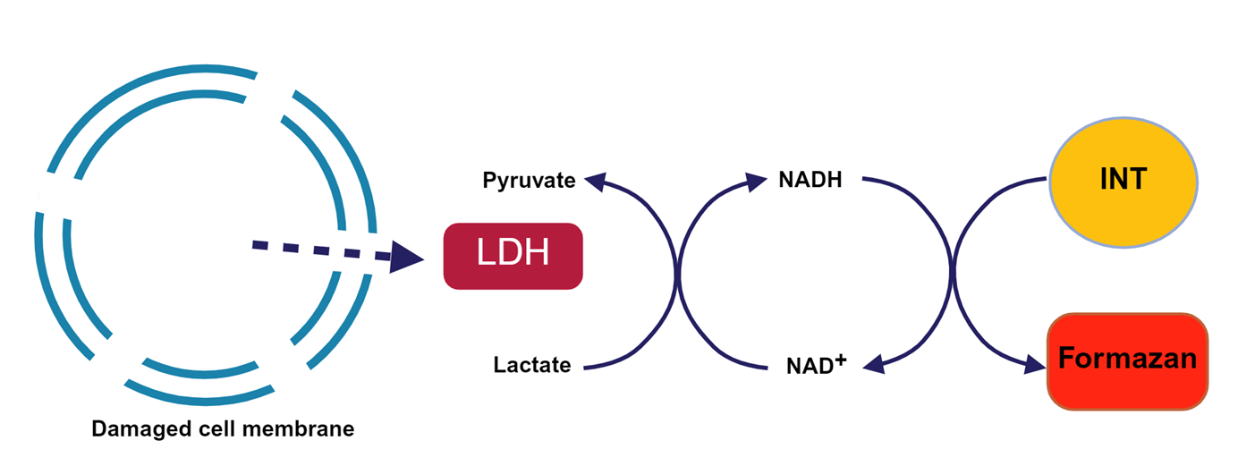
Figure1. Principle of LDH Assay

Method

The cytotoxicity function of CAR-NK cells was assessed by co-culture tumor cells at an E:T (effector to target) ratio of 1:1. For lactate dehydrogenase (LDH), CytoTox96 cytotoxicity assay was used according to the manufacturer’s instructions (Promega, G1780).

Cytotoxicity (%) = [LDHE:T -LDHE]/LDHMax × 100%

A. Cell Preparation:

1. Seed K562 cells and previously proliferated NK cells into culture dishes with the appropriate medium. For the experimental group, use medium supplemented with 15 mM lactic acid to adjust the pH to 6.4; for the control group, use medium with pH 7.4. Incubate at 37°C with 5% CO₂ for 36 h. Change to a fresh medium the evening before the experiment.

B. Cytotoxicity Assay:

1. A 96-well round-bottom plate was prepared for the cytotoxicity assay. Experiments were conducted at E:T ratios of 1:1 , with replicates per ratio. Effector and target cells were added to each well, with a total volume of 100μL per well.

2. Control wells were set up: Natural release control wells with the same number of effector cells as in the experimental wells. Maximum release control wells with the same number of target cells, adding medium to achieve a final volume of 90 µL per well. Natural release control wells for target cells, adding medium to achieve a final volume of 100 µL per well. Background control wells with 100 µL of CAR-NK cells.

Wells	Cell types	Volume (per well)
Experimental Wells	Effector and target cells	100 μL
Natural release control wells	Effector cells	100 μL
Maximum release control wells	Target cells	90 µL
Natural release control wells	Target cells	100 μL
Background control wells	NK cells	100 μL

3. 10μL of sterile ultrapure water was added to the spontaneous Release Control wells for both effector and target cells. Spontaneous Release Control wells were built to reduce the interference of non-specific release from cells under normal culture conditions on the experimental results.

4. The plate was incubated at 37°C with 5% CO₂ for 4 hours.

5. 10 μL of lysis buffer was added to the Maximum Release Control wells and incubated for 45 minutes.

6. The plate was centrifuged at 250 g for 3 minutes. 50 μL of supernatant was transferred from each well to a corresponding flat-bottom plate. 50 μL of reaction substrate was added to each well and incubated in the dark at room temperature (25°C) for 30 minutes. Once color developed, 50 μL of stop solution was added to each well and the plate was mixed gently.

7. A microplate reader was used to measure the absorbance at 490 nm and 680 nm. Subtract the absorbance value at 680 nm (background signal) from the absorbance at 490 nm (D).

8. For accurate calculations, the average Background Control value was subtracted from the average experimental value, the Effector Cell Spontaneous Release Control value, and the Target cell spontaneous release control value.

9. The NK cell killing rate (%) was calculated using the following formula:

NK killing Rate(%) = (Exp OD - Eff Spont OD - Tgt Spont OD - Bkgd Avg)/(Max Release OD - Tgt Spont OD)×100%

Lysis Rate(%) = (Exp LDH - Tgt Spont LDH)/(Max Release LDH)  ×100%